Example - Running the fetal model with an anatomical placenta
This example is found in the directory placenta-simulations/fetal/fetal_example
The example requires that you have the reprosim libraries installed on your machine. You can find installation instructions here and the libraries themselves here.
If you work in virtual environments, activate a virtual environment in which reprosim is installed and execute the following:
You will also need to make sure you have the following python libraries installed:
numpy
placentagen (found here)
csv
matplotlib
python run_fetal.py
This executes the file that runs the example (run_fetal.py). If you open this file you’ll see that the code has a requirement
import os
import numpy as np
import placentagen as pg
import csv
from matplotlib import pyplot as plt
These are packages you should have installed on your computer. The os package often comes with your python install, but if not can be installed using pip.
The next lines of code tell you which parts of the reprosim libraries we are going to use:
from reprosim.diagnostics import set_diagnostics_level
from reprosim.indices import perfusion_indices, get_ne_radius
from reprosim.geometry import append_units,define_node_geometry, define_1d_element_geometry,define_1d_element_placenta,define_rad_from_geom,add_matching_mesh, \
    define_capillary_model,define_rad_from_file
from reprosim.repro_exports import export_1d_elem_geometry, export_node_geometry, export_1d_elem_field,export_node_field,export_terminal_perfusion
from reprosim.fetal import assign_fetal_arrays, fetal_model
The next portion of the code sets up the parameterisation of the model, parameters related to the heart are defined directly within the python script, and the geometry (nodes and elements that define the vascular connectivity in the fetal circulation) is defined within two spreadsheets (.csv) files that need to be imported into reprosim libraries for the models to function.
The first lines of code are here to allow you to define the directory you want to export results to, they define the directory name, and if it doesnt exist on your system creates the directory.
export_directory = 'output'
if not os.path.exists(export_directory):
    os.makedirs(export_directory)
Next, there are a number of numeric parameters that define the running of the model and the fetal heart model employed
In this example, the numerical scheme will use a time step of 0.0001 s and simulate for 30 heart beats, evolving from initial conditions.
The model parameters that relate to the heart are as follows:
T_beat = 0.43 # heart beat period (s)
T_vs  = 0.215 # Time period of ventricular contraction (s)
T_as = 0.1075 #Time period of atrial contraction (s)
T_v_delay = 0.1075 #delay in ventrial contraction (compare to atria) (s)
U0RV = 5332.89 #Pa
EsysRV = 0.399967 #Pa/mm3
EdiaRV = 0.0399967 #Pa/mm3
RvRV = 0.010665 #Pa.s/mm3
U0LV = 5332.89 #Pa
EsysLV =0.399967 #Pa/mm3
EdiaLV =0.0399967 #Pa/mm3
RvLV = 0.010665 #Pa.s/mm3
U0A = 399.967 #Pa
V0V = 8000.  # mm3 - volume of ventricles (initial)
V0A = 3000.  # mm3 - volume of atria (initial)
human_weight = 3.0255 #kg Not used, but current parameterisation assumes an average fetal weight and allometric scaling may be useful in future
Next, the code reads in a .csv file defining element properties:
elem_file = 'elemProperties.csv'
file = open(elem_file)
elem_properties = csv.reader(file)
header = next(elem_properties)
rows = []
for row in elem_properties:
    rows.append(row)
file.close()
elem_identifiers = np.empty(len(rows),dtype=np.dtype('U10'))
elems = np.empty((len(rows),3),dtype=int)
group = np.empty(len(rows),dtype=int)
resistance = np.empty(len(rows),dtype=np.dtype('d'))
L= np.empty(len(rows),dtype=np.dtype('d'))
K = np.empty(len(rows),dtype=np.dtype('d'))
for i in range(0,len(rows)):
    elem_identifiers[i] = rows[i][0]
    elems[i,0]=int(rows[i][1])-1
    elems[i,1]=int(rows[i][2])-1
    elems[i,2]=int(rows[i][3])-1
    resistance[i]=np.double(rows[i][header.index('R')])
    group[i]=int(rows[i][header.index('group')])
    L[i]=np.double(rows[i][header.index('L')])
    K[i]=np.double(rows[i][header.index('K')])
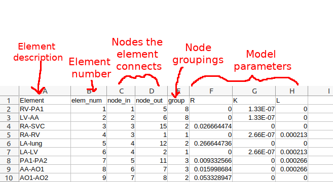
The contents of elemProperties.csv.
Of importance to how the model works is the element groupings defined in elemProperties.csv. These are:
Cardiac valves.
A resistor only element, not connected to the placenta
A resistor combined with an inductor
The foramen ovale.
A resistor combined with a flow dependent dissipation.
A resistor combined with a flow dependent dissipation and an inductor.
Elements that feed the circulation from the heart (exits the ventricles).
A dummy argument to allow for future additions to the model (do not use).
The umbilical artery (feeding the anatomic placenta). A resistor only element.
The umbilical vein (exiting the anatomic placenta). A resistor only element.
Next, each element’s properties are converted to reprosim (and cmgui) readable files:
pg.export_ipelem_1d(elems, 'fetal', export_directory + '/fetal')
pg.export_exfield_1d_linear(resistance, 'fetal', 'resistance', export_directory +'/R')
pg.export_exfield_1d_linear(group, 'fetal', 'group', export_directory + '/group')
pg.export_exfield_1d_linear(L, 'fetal', 'L', export_directory + '/L')
pg.export_exfield_1d_linear(K, 'fetal', 'K', export_directory + '/K')
The node properties are now read into the code and converted into reprosim readable files:
node_file = 'nodeProperties.csv'
file = open(node_file)
node_properties = csv.reader(file)
header = next(node_properties)
rows = []
for row in node_properties:
    rows.append(row)
file.close()
nodes = np.empty((len(rows),4),dtype=np.dtype('d'))
node_identifiers = np.empty(len(rows),dtype=np.dtype('U10'))
for i in range(0,len(rows)):
    node_identifiers[i] = rows[i][0]
    nodes[i,0]=np.double(rows[i][1])-1
    nodes[i,1]=np.double(rows[i][header.index('group')])
    nodes[i,2]=np.double(rows[i][header.index('press')])
    nodes[i,3]=np.double(rows[i][header.index('comp')])

pg.export_ip_coords(nodes[:,1:4], 'fetal', export_directory +'/fetal')

The contents of nodeProperties.csv.
Just like with element groups, the node groups in nodeProperties.csv are important. They are defined as:
Right ventricle
Left ventricle
Atria
All other vessels or vascular beds
The main portion of the code comes next. Within reprosim, we can chose how much diagnostic information we want to print to screen as we run the code. Thre are three levels of diagnostics (level 0 - no diagnostics; level 1 - only prints subroutine names (default); level 2 - prints subroutine names and contents of variables). To set this level we simply use:
set_diagnostics_level(0)
We then set up a perfusion model type - this part of the code simply tells the solver we are looking at a perfusion simulation and allows it to determine how much memory is needed to do this:
perfusion_indices()
Next we set up the geometry that we are going to solve the model in. The first thing we read in is the fetal circulation architecture which has been converted from csv files to be reprosim readable:
define_node_geometry(export_directory +'/fetal.ipnode')
define_1d_element_geometry(export_directory + '/fetal.ipelem')
assign_fetal_arrays()
We then need to define the placenta itself. This involves reading in, or generating a tree-like structure. In this example we read in a geometry from the ‘sample_geometry’ directory:
define_node_geometry('sample_geometry/FullTree.ipnode')
define_1d_element_placenta('sample_geometry/FullTree.ipelem')
    append_units()
Here, nodes are the location of the start and end points of branches in our geometry and elements define the centrelines of these branches. The append_units command tells the code where our capillary bed sits within our geometry.
In many cases we have a really good description of what our arteral geometry looks like, but we need to make some assumptions about what the veins look like. In this case we simply copy the arteries:
umbilical_elem_option = 'same_as_arterial'
umbilical_elements = []
add_matching_mesh(umbilical_elem_option,umbilical_elements)
We now have a mesh that includes arteries, capillaries and veins, and we have to define the size of these vessels. We do this using Strahler ordering systems:
# define radius by Strahler order in diverging (arterial mesh)
s_ratio = 1.38  # rate of decrease in radius at each order of the arterial tree  1.38
inlet_rad = 1.8  # inlet radius
order_system = 'strahler'
order_options = 'arterial'
name = 'inlet'
define_rad_from_geom(order_system, s_ratio, name, inlet_rad, order_options, '')
#defines radius by STrahler order in converging (venous mesh)
s_ratio_ven= 1.46 #rate of decrease in radius at each order of the venous tree 1.46
inlet_rad_ven=4.0 #inlet radius
order_system = 'strahler'
order_options = 'venous'
first_ven_no='' #number of elements read in plus one
last_ven_no='' #2x the original number of elements + number of connections
define_rad_from_geom(order_system, s_ratio_ven, first_ven_no, inlet_rad_ven, order_options,last_ven_no)

num_convolutes = 6  # number of terminal convolute connections
num_generations = 3  # number of generations of symmetric intermediate villous trees
calc_capillary_unit_length(num_convolutes,num_generations)
Finally, we solve the model (bringing in information about heart and where to export files):
fetal_model(export_directory+'/',dt,num_heart_beats,T_beat,T_vs,T_as,T_v_delay,U0RV,EsysRV,EdiaRV,RvRV,U0LV,EsysLV,EdiaLV,RvLV,U0A,V0V,V0A)
The remainder of the code exports provides some plots of blood flow velocity in major vessels. Examples of these plots are given in the expected-results folder.