Example - Model from Clark Whitfield et al. 2024, whole placenta nutrient exchange

This example describes a feto-placental nutrient transport model, which predicts the distribution of exchange and nurtrient uptake in an anatomical feto-placental geometry.

This example is found in the directory placenta-simulations/fetoplacental/nutrient_transport

Requirements

The example requires that you have the reprosim libraries installed on your machine. You can find installation instructions here and the libraries themselves here.

You need to have python installed, and Julia (https://julialang.org/). Make sure you add the Julia install to PATH.

You also need to properly install pyjulia (note that this is more complicated than a simple pip install).

You will need other python libraries. These are listed under pyrequirements.txt in the model example directory.

Within Julia you will need to do the following:

import Pkg
Pkg.add("SpecialFunctions")
Pkg.add("Distributions")

Step 1 - run perfusion models

There is a shell script provided to run the perfusion model multiple times under a range of different inlet flow conditions. The shell script is called: step1_run_multiple_bloodflow.sh

To run the shell script simply type into a terminal:

./step1_run_multiple_bloodflow.sh

Inside the shell script you will find a series of terminal commands. First we generate a list of inlet blood flows (in ml/min) that we want to simulate, and then we loop through this list and run the run-bloodflow.py script multiple times with inlet arguments $i for flow, and 0.0 for fractional vessel occlusion (this allows us to manipulate vessels by blocking then off). In this example we keep the screen dumps from running the python script in a text file and move these text files to the output directory when we run the python script. Finally, we move all out model outputs to a single output directory for processing.

list=(20.0 40.0 50.0 60.0 80.0 100.0 150.0 200.0 250.0 300.0 350.0 400.0 450.0 500.0)
for i in ${list[@]}
do
    echo $i
    python run-bloodflow.py $i 0.0  > screen_$i.txt
    mv screen_$i.txt output_flowbc_${i}ml_min_0.0
done
mkdir output-normal
mv output_flowbc_* output-normal/.

The main bulk of the python script run-bloodflow.py is described in other examples. Here we just run through the main differences compared to what has been considered before. First, our python script has input arguements:

blood_flow_ml = float(args[0])
remove_frac = float(args[1])
blood_flow_model_units = blood_flow_ml / 60. * 1000.
print(blood_flow_ml, blood_flow_model_units, remove_frac)

In python these are defined as args. The first argument is inlet blood flow in ml/min (converted to model units of mm:math:^3/min in the python code, and the second gives the option to remove some fraction of vessels of a given Strahler order at random. By default we use 0.0 here, unless we want to manipulate and remove vessels.

We use a new capillary model ‘erlich resistance’ which instructs reprosim to use terminal villous resistance in perfusion simulations following prior studies based on anatomical imaging.

capillary_model = 'erlich_resistance'

We also set rheology and vessel types to reflect a non-linear (Pries model) rheology, and compliant vessels:

rheology_type = 'pries_vessel'
vessel_type = 'elastic'

Finally, if we had included a non-zero fraction of vessels to occlude, we could instruct reprosim to do this, at any given Strahler order, if you are interested you can change the occlusion fraction and Strahler order to explore effects of doing this.

if remove_frac > 0.0:
    print("Occluding order 6 vessels")
    update_radius_by_order(6, 0.01, 'random', remove_frac)

Running the shell script will create a host of files in the output-normal directory:

output_flowbc_100.0ml_min_0.0       output_flowbc_40.0ml_min_0.0
output_flowbc_150.0ml_min_0.0       output_flowbc_400.0ml_min_0.0
output_flowbc_20.0ml_min_0.0        output_flowbc_450.0ml_min_0.0
output_flowbc_200.0ml_min_0.0       output_flowbc_50.0ml_min_0.0
output_flowbc_250.0ml_min_0.0       output_flowbc_500.0ml_min_0.0
output_flowbc_300.0ml_min_0.0       output_flowbc_60.0ml_min_0.0
output_flowbc_350.0ml_min_0.0       output_flowbc_80.0ml_min_0.0

Step 2 - convert perfusion model outputs to nutrient transport model inputs

This step is currently required to convert University of Auckland perfusion model outputs to University of Manchester exchange model inputs. In a console simply run:

python step2_data_conversion.py

This script will create two files in your output-normal directory:

tree_flux_sweep.pbz2
tree_flux_sweep_terminal.pbz2

Step 3 - run nutrient transport model

The next step is to run the nutrient transport model:

python step3_nutrienttransport.py

First we import required python packages, including the julia code which solves the model:

from julia import Main
Main.include("./scripts/calculate_villous_fluxes.jl")
import numpy as np
import sys
sys.path.append('./scripts')
import placenta_calculations as pcalc

Next, we need to define output diretories, the inlet flux values we are intterested in, and properties of the placental micro-vascular tree

TreeFilenames = ["normal"]
outputdir = 'output-normal/'
inputdir = outputdir
flux_vals = np.array([20,40,60,80,100,150,200,250,300,350,400,450,500],dtype=float)
Nparallel = 1        #Number of convolute units in parallel
Nseries = 3          #Number of terminal villi in a row from a single mature intermediate villous
Nparallel_cap = 1    #Number of parallel capillaries in an imaged convolute (leiser), typically 1
Nconv = 10       #as per leiser 10 terminal conduits in a single feeding vessel (typically 10)
Ngens = 3   #Typically 3
tree_path = outputdir+'/tree_flux_sweep.pbz2'
term_path = outputdir+'/tree_flux_sweep_terminal.pbz2'
villous_flux_dir = outputdir

We load in our terminal flow results from our perdusion simulations:

term_props = Main.load_pickle(decompress(term_path))

and we calculate nutrient flux for each terminal unit, under each flow condition:

Main.calculate_and_save_allfluxes(outputdir,
                term_props[0], TreeFilenames, flux_vals,
                Nparallel, Nseries, Nparallel_cap, Nconv, Ngens, use_full_res=True)

Finally we calculate and save all model output measures interest, at any given flow inlet value (here 250 ml/min)

vtk_print_fluxes = np.array([250])    #flux value to produce vtk file for
pcalc.calculate_and_save_measures(outputdir+"/flux_sweep_outcomes.pkl", \
    tree_path, term_path, villous_flux_dir, ['normal'], ['normal'], \
    pcalc.SoluteNames, pcalc.DC, pcalc.B, pcalc.Dt, Nparallel, Nseries, Nparallel_cap, Nconv, Ngens, \
    vtk_print_fluxes)

Your output-normal directory should now contain a number of files and sub-directories:

normal_np1ns3_flux_250_term.vtk     tree_flux_sweep.pbz2
normal_np1ns3_flux_250_tree.vtk     tree_flux_sweep_terminal.pbz2
output_flowbc_100.0ml_min_0.0       tv_fluxes_normal_flow100.pkl
output_flowbc_150.0ml_min_0.0       tv_fluxes_normal_flow150.pkl
output_flowbc_20.0ml_min_0.0        tv_fluxes_normal_flow20.pkl
output_flowbc_200.0ml_min_0.0       tv_fluxes_normal_flow200.pkl
output_flowbc_250.0ml_min_0.0       tv_fluxes_normal_flow250.pkl
output_flowbc_300.0ml_min_0.0       tv_fluxes_normal_flow300.pkl
output_flowbc_350.0ml_min_0.0       tv_fluxes_normal_flow350.pkl
output_flowbc_40.0ml_min_0.0        tv_fluxes_normal_flow40.pkl
output_flowbc_400.0ml_min_0.0       tv_fluxes_normal_flow400.pkl
output_flowbc_450.0ml_min_0.0       tv_fluxes_normal_flow450.pkl
output_flowbc_50.0ml_min_0.0        tv_fluxes_normal_flow500.pkl
output_flowbc_500.0ml_min_0.0       tv_fluxes_normal_flow60.pkl
output_flowbc_60.0ml_min_0.0        tv_fluxes_normal_flow80.pkl

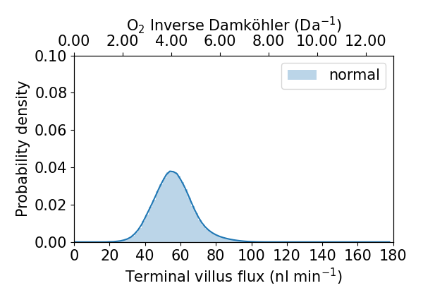
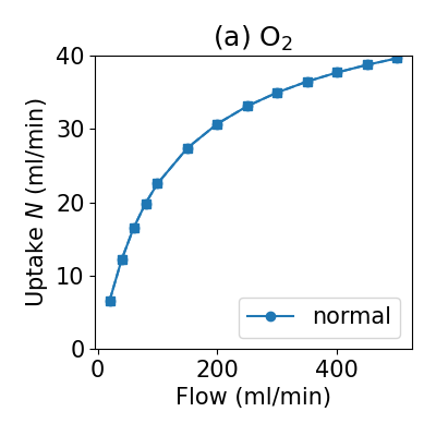
Step 4 - plot some results!

Now, we get to look at results, note that when you become familiar with data structures you will be able to plot results however you see fit.

python step4_plotting.py

This will produce two png figures in your output-normal directory