Characterising the Gross Morphology of a Tissue Block

This example is found in the directory placenta-simulations/imageprocessing/morphology

The example requires that you have numpy installed on your machine, and the placentagen libraries.

If you work in virtual environments, activate a virtual environment in which placentagen is installed and execute the following:

python gross_morphology.py

This executes the file that runs the example (gross-morphology.py). If you open this file you’ll see that the code has a number of requirements

import SimpleITK as sitk
import networkx as nx
import numpy as np
from skan.csr import skeleton_to_csgraph
from scipy.stats import variation
import copy
import skimage as sk
import os

These are the packages you should have installed on your computer. For os and numpy, these often come with your python install, but if not can be installed using pip. The package placentagen is developed in house, and details on how to install can be found at this link. Skan, scipy, and skimage can be installed with pip.

Once you are confident that you have all these packages installed, run the script. The results should write to a new directory (output), where a number of parameters are written out.

Villous CCMP: 1
Intervillous CCMP: 652
Area: 3897393.2800000007
Volume: 48150621.18400001
Porosity: 0.698545968876719
Number of Terminal Branches: 2944
Number of Branch points: 2944
Number of Cycles: 2513
Fractal Dimension: 2.9248030002530427
Lacunarity: 0.33857695497797347

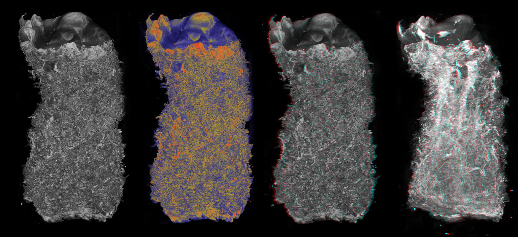
The parameters from the sample dataset have been written above. The dataset is from here, and has labels of 1 for villous tissue, and 2 for arterial vessels. In this exampe we will consider the aggregate villous tissue as a label of 1, and it is anywhere in the dataset where the value of a voxel is greater than 0.

The first two parameters deal with the number of distinctly connected components in the images. The connectivity we use here is ‘6-connectivity’, or ‘face connectivity’, where voxels of the same value are defined to be connected if they share a face.

Villous CCMP is the number of distinctly connected components that have been labelled as villous tissue, while intervillous CCMP is the number of distinctly connected components in the intervillous space.

The next three parameters deal with gross geometric qualities of the villous tissue, namely the tissue volume, the villous surface area, and the volume fraction or porosity. The surface area is calculated by adding up the sum of villous voxel faces exposed to the intervillous space (exposed to voxels with a value of 0). The porosity is the fraction of the image volume that is villous tissue.

The next three parameters look at characterising the branching properties of the villous skeleton. The skeleton is a representation of the villous centreline, and represents the net connective information within the villous segmentation. We consider the skeleton as a graph structure where voxels in the skeleton become nodes in the graph, with face - face connections between voxels being represented as an edge between nodes. In this representation, branches are collections nodes that form a vessel. In the graph representation, node degree is the number of edges that attach to a particular node. Nodes of degree one are terminal nodes, and connect to only one other node. Nodes of degree two, connect to two other nodes and are the main node type you get in branches. Higher degree nodes, have a degree of 3 or higher, and are called branch nodes. Using the node degree definition, we can say that a branch is a collection of degree 2 nodes, that connect either two branch nodes, or one branch node and one terminal node.

The number of cycles is the number of sets of branches in the graph representation of villous tissue connectivity that form loops.

The next two parameters look at characterising the relationship between scale and complexity using the Fractal Dimension , and the spatial heterogeneity, or gappipness, using Lacunarity.